
MathLive User Guide
Overview
This page is not a traditional “user guide” in the strict sense. Instead, it serves as a collection of example problems designed to showcase MathLive’s capabilities and help users become familiar with how to enter functions, manipulate the graph, and activate features such as intersection detection.
The examples chosen are often equations that are difficult—or impossible—to solve in elementary closed form. By exploring these examples, users can see how MathLive can be used to visualize multiple functions, identify where two or more functions intersect, and therefore determine the solution points of the given equations.
This approach not only illustrates the power of MathLive’s graphing and intersection tools but also provides a hands-on way to learn and practice solving mathematical problems numerically. Please note that this 2D grapher — the 2D Function Graphing Calculator and Visual Equation Solver — finds solutions only for functions in the real number field \(\mathbb{R}\). It will not solve problems for implicit equations involving both \(x\) and \(y\) in the same equation, where the relationship cannot be expressed as \(y = g(x)\). For example, \(x^2 + y^2 = 1\) (circle), \(x^2 - y^2 = 4\) (hyperbola), or in general form \(F(x, y) = 0\). Future revisions of MathLive may include the ability to solve and plot implicit equations.
1. Transcendental equations
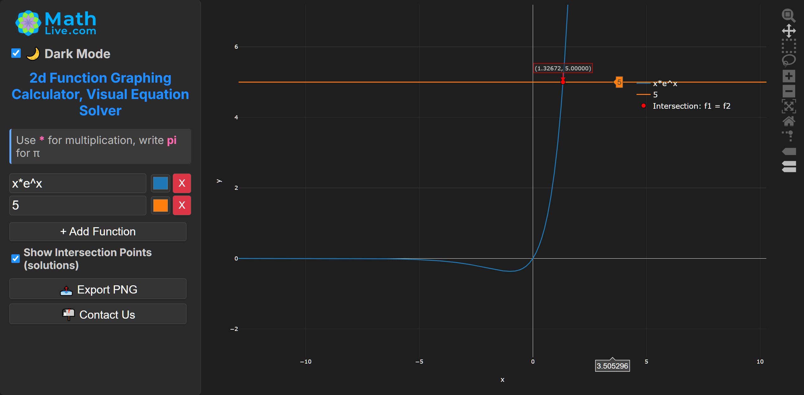
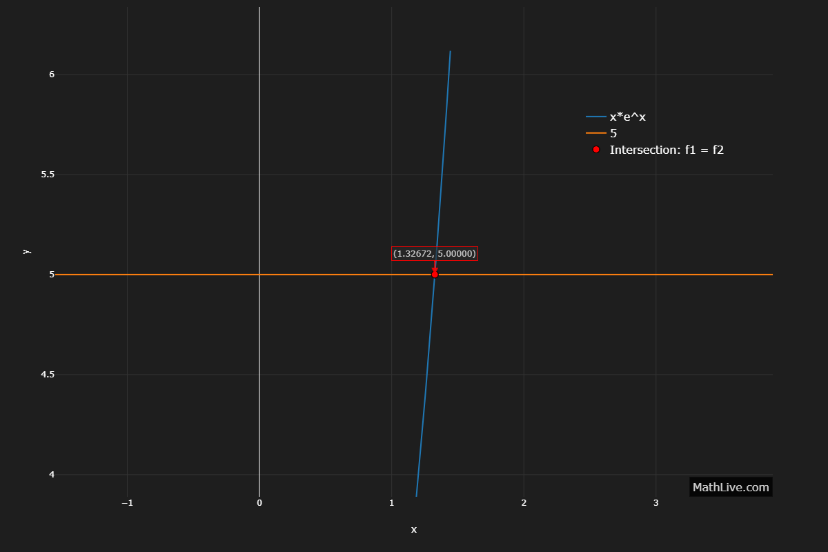
No elementary closed form; solution via the Lambert \( \operatorname{W} \) function: \( x = \operatorname{W}(5) \approx 1.32672466 \).
Numerically: MathLive.com uses bisection method to solve \( x e^{x} = 5 \).
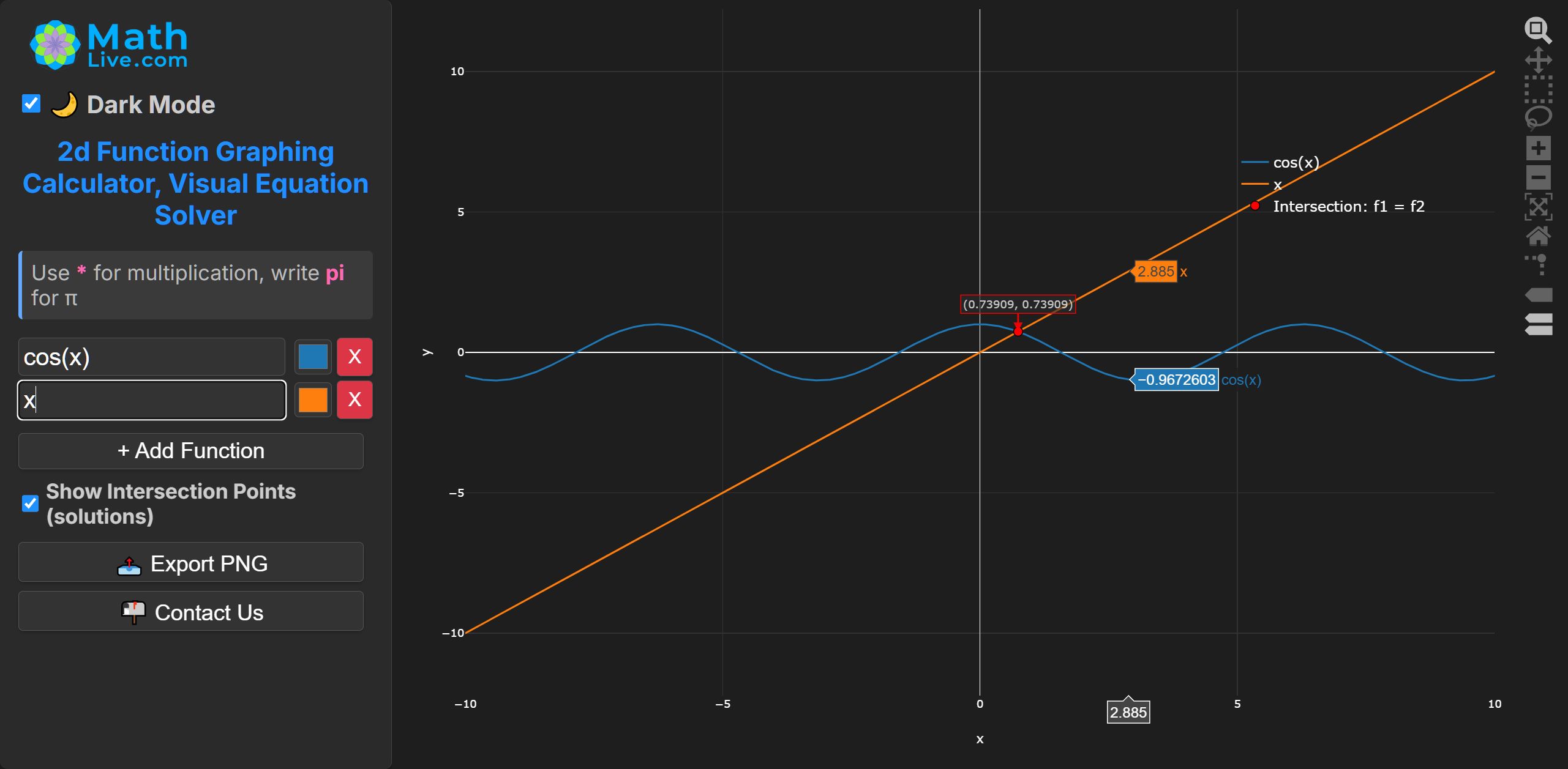
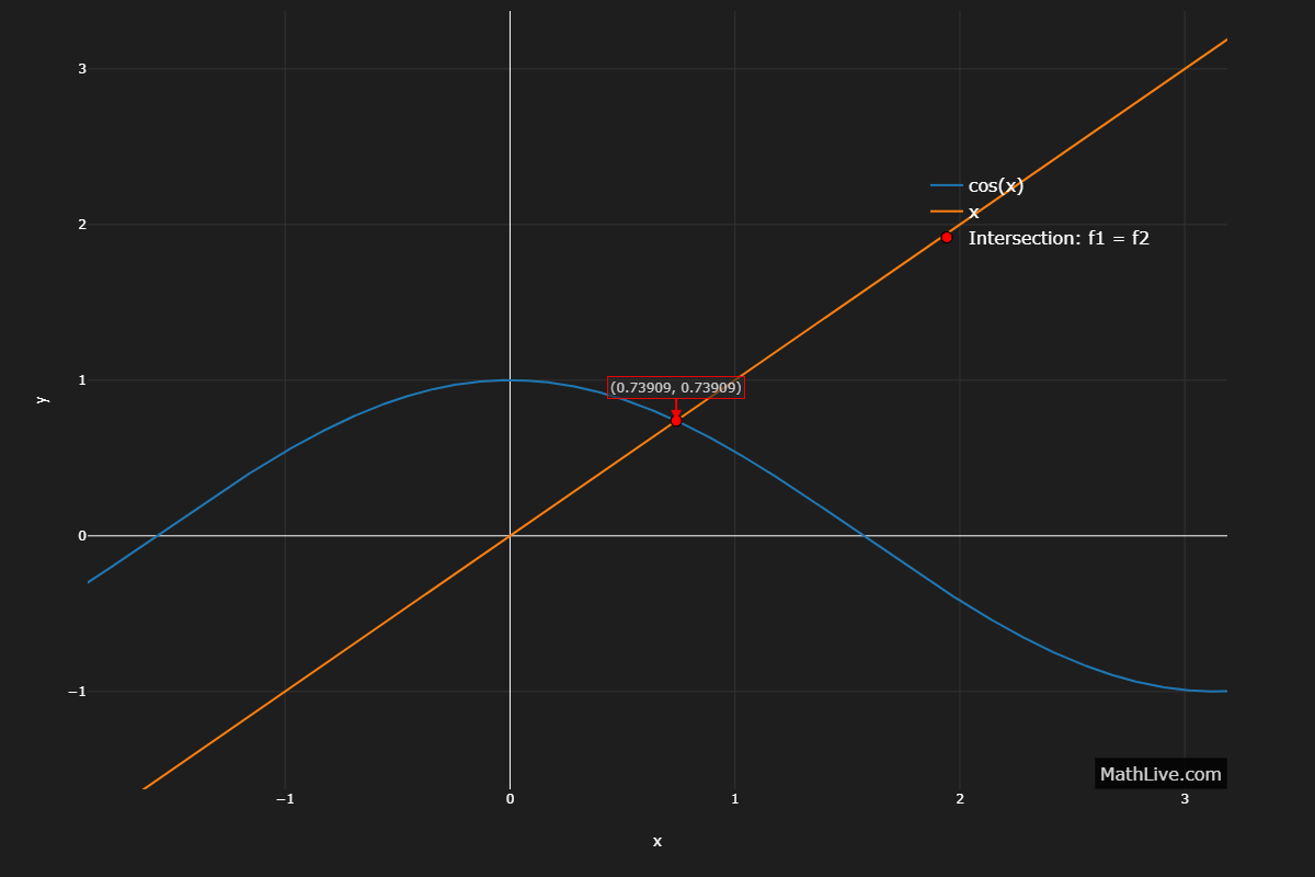
No closed form. One real root near \( x \approx 0.739085 \).
MathLive.com uses bisection method to solve \( \cos x = x \).
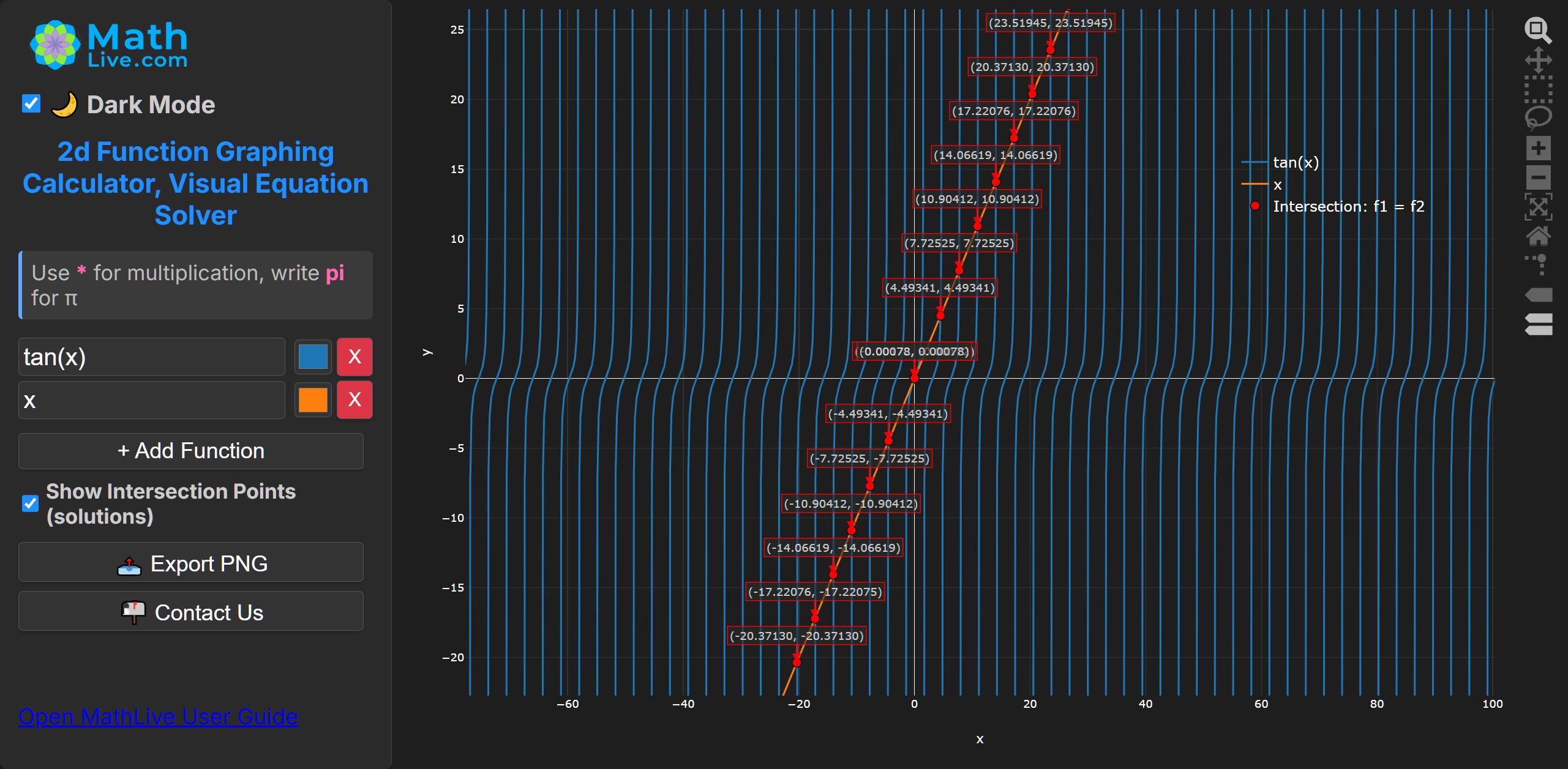
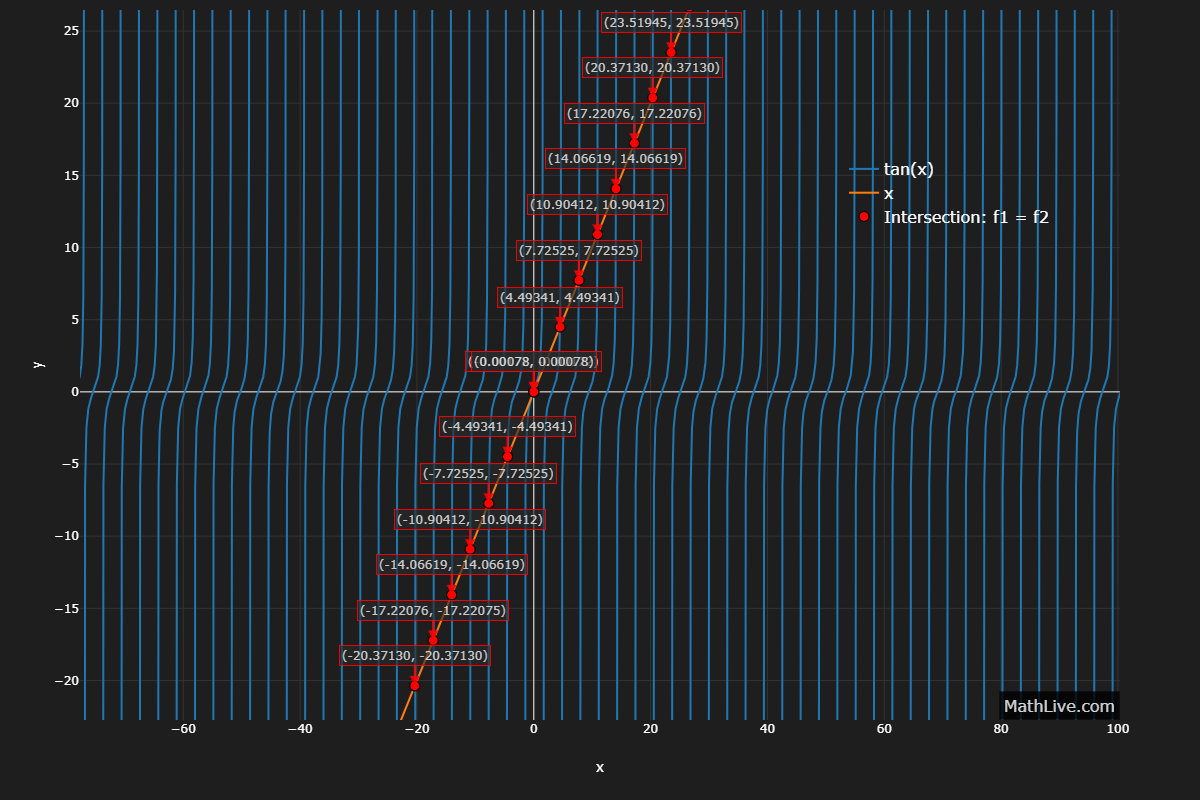
Infinitely many roots; none in \( (-\tfrac{\pi}{2},0) \), one near \( 0 \), and one in each interval \( (k\pi-\tfrac{\pi}{2},\,k\pi+\tfrac{\pi}{2}) \). Use bracketing + Newton for each interval.
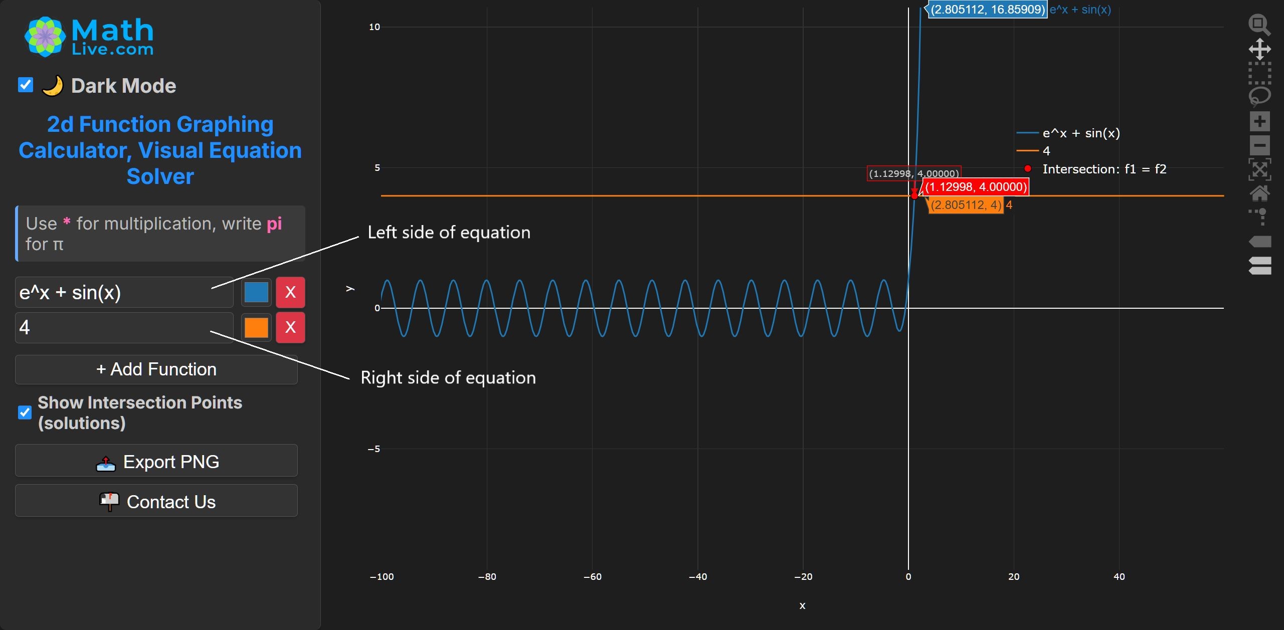
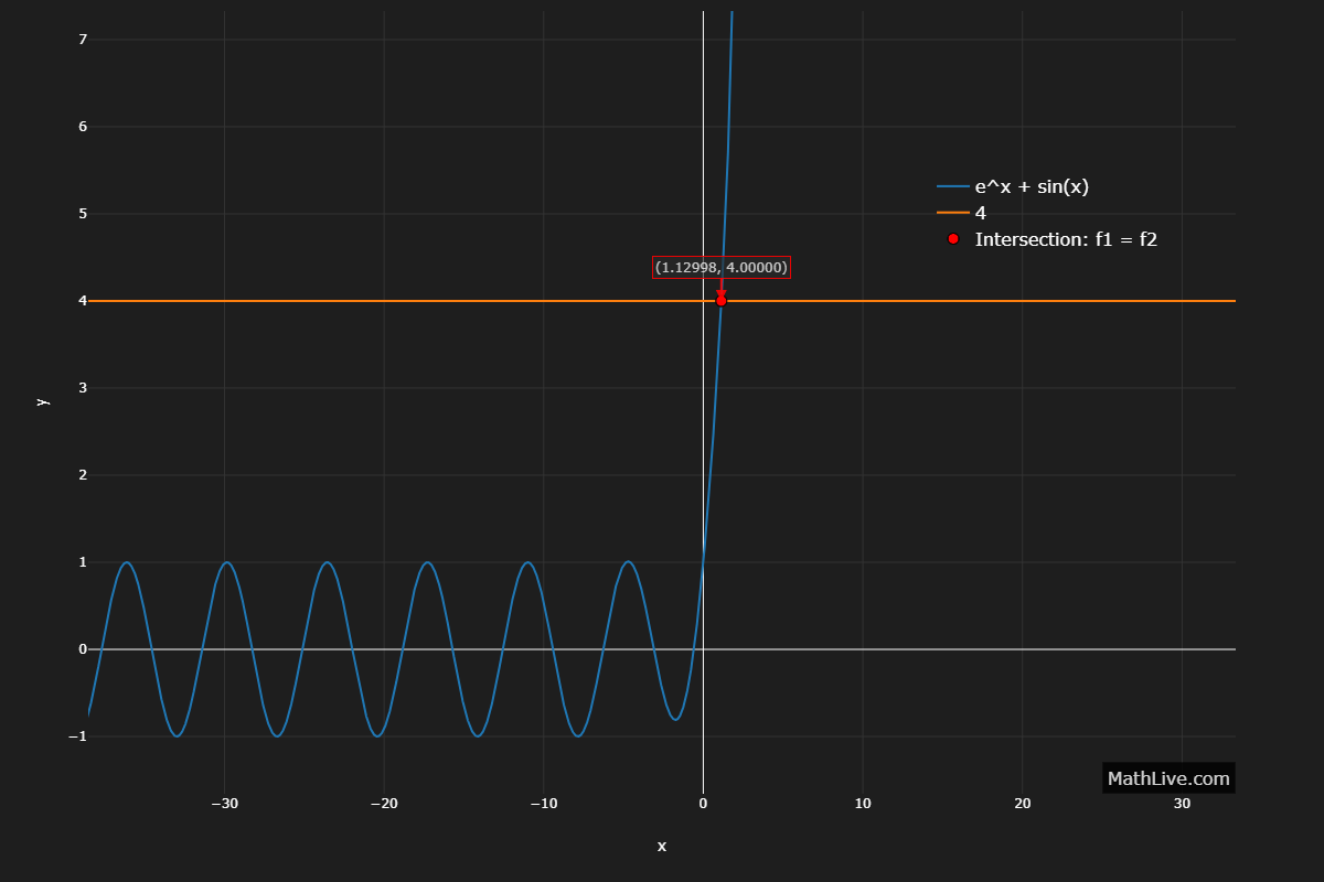
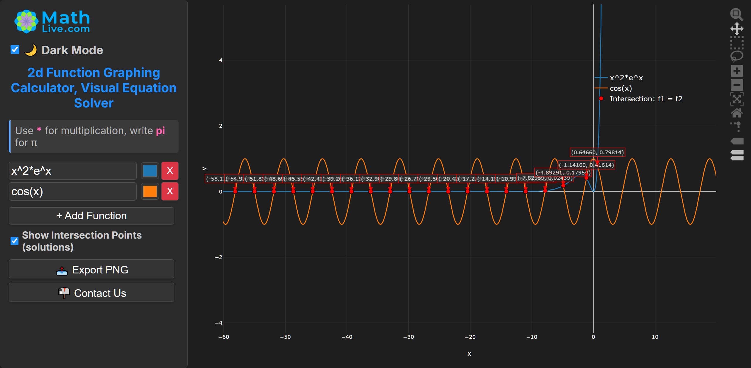
2. Mixed trigonometric–exponential
No closed form. Unique real root near \( x \approx 1.1299805 \).
Use bisection on \( [1,1.2] \) or Newton with \( f'(x)=e^x+\cos x \).
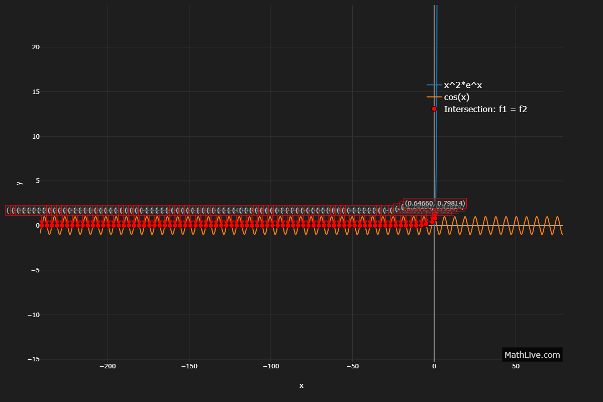
Infinitely many real roots accumulating for large negative \( x \).
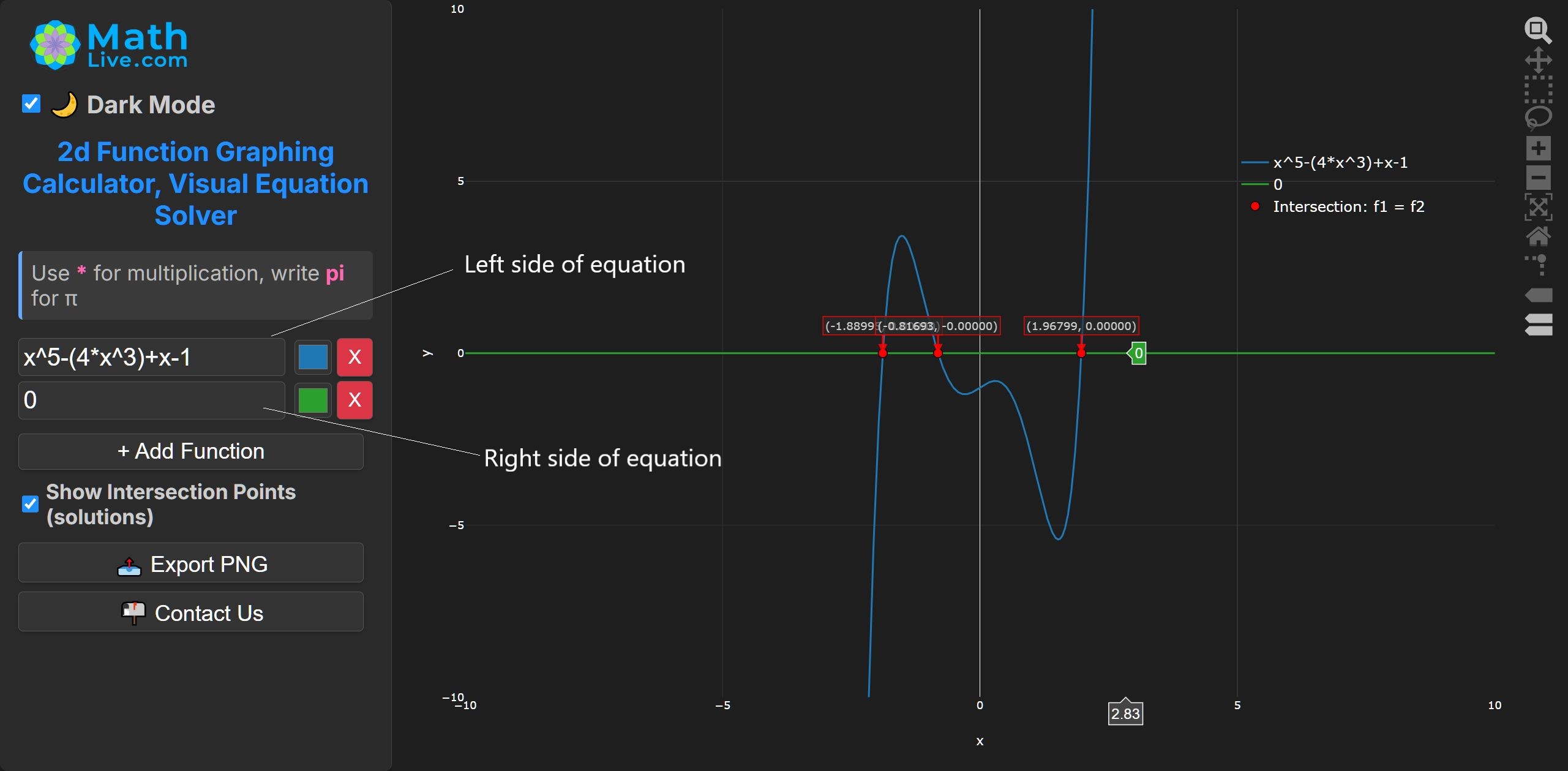
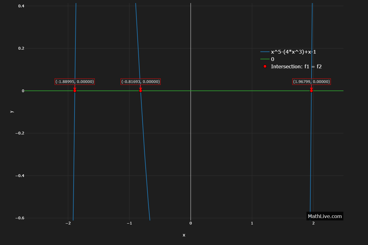
3. Fifth-degree polynomial
\( x^{5} - 4x^{3} + x - 1 = 0. \)
By Abel–Ruffini, no general radicals solution.
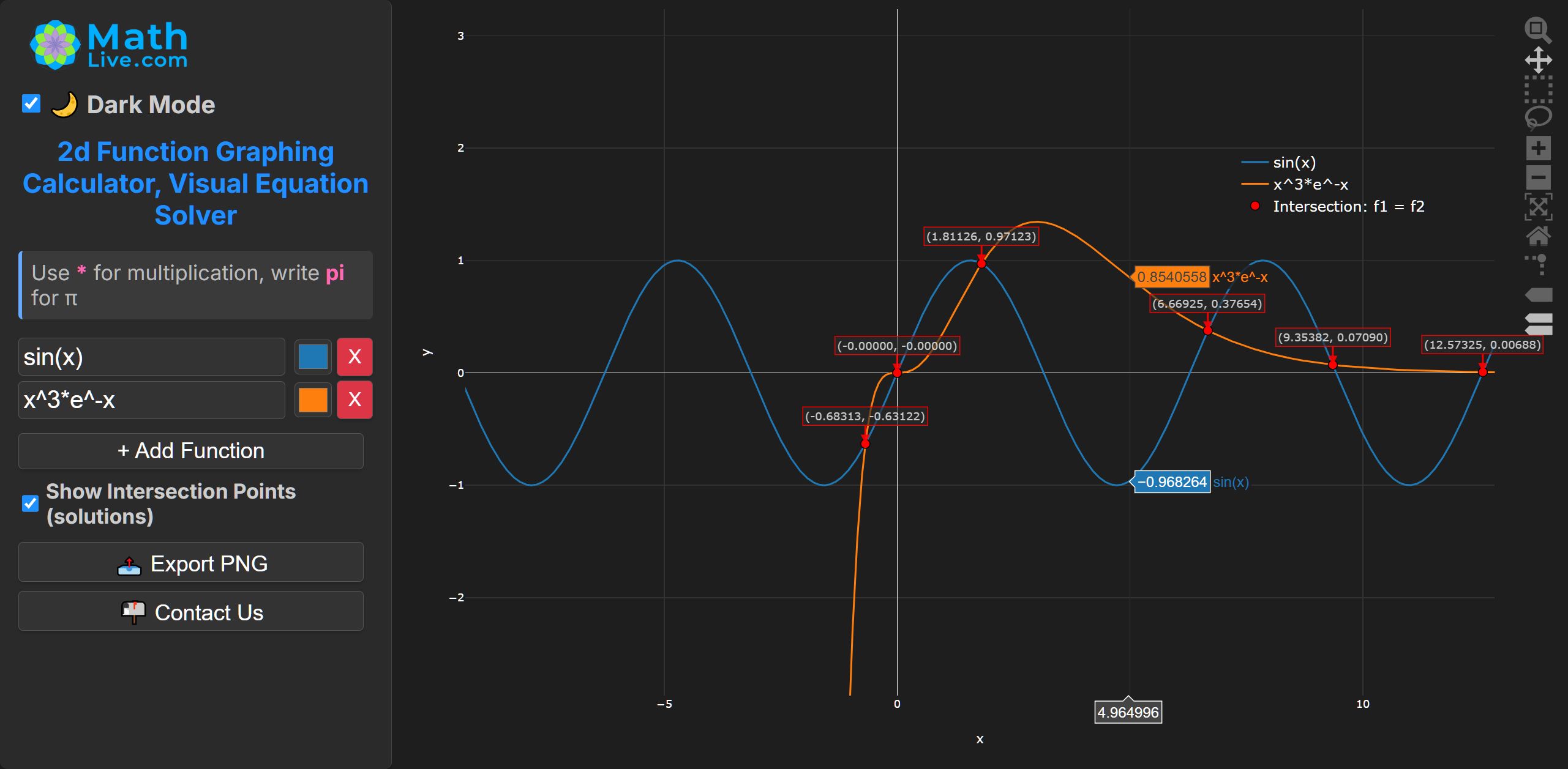
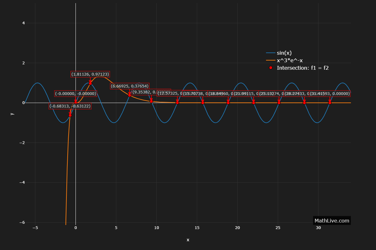
4. Complex transcendental form
\( \sin x = x^{3} e^{-x}. \)
Many crossings; bracket each sign change and refine by bisection.
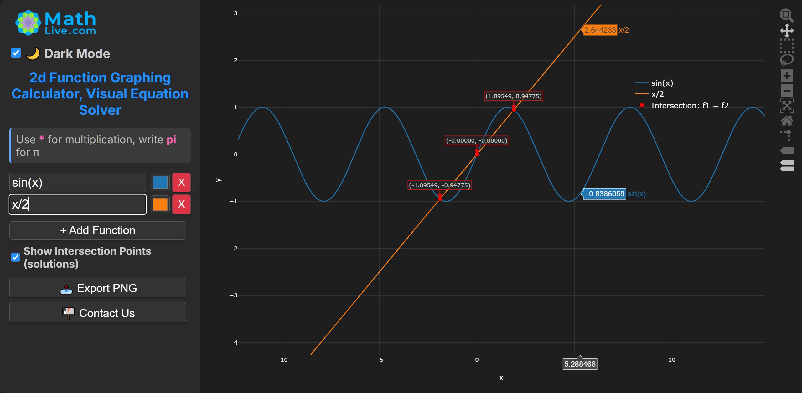
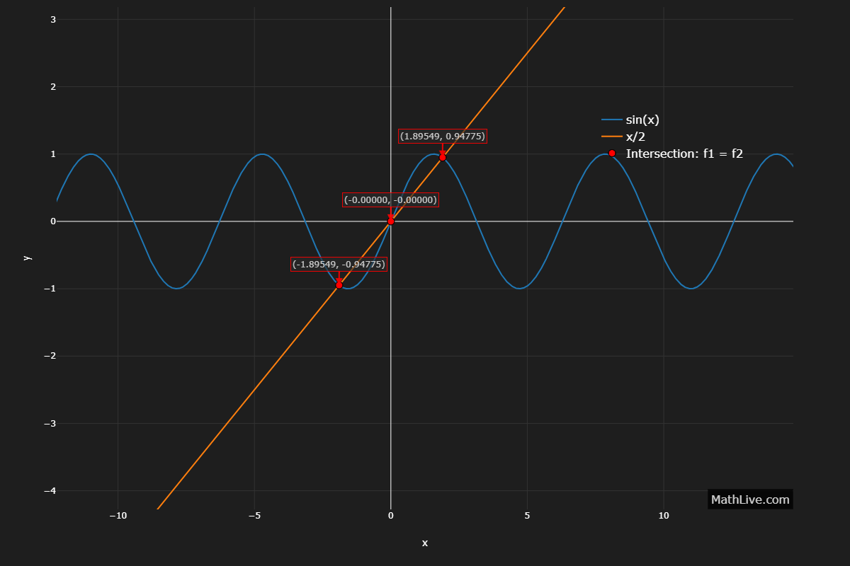
5. Nonlinear eigenvalue problem
\[ \sin \lambda = \frac{\lambda}{2} \]
Discrete spectrum of \( \lambda \). Solve per interval with bracketing
Notes on MathLive Method to Find Intersections (Solutions)
MathLive uses the Bisection Method to find the coordinates of intersection points between functions. This numerical method is guaranteed to find a root if the function values at the endpoints \(a\) and \(b\) have opposite signs (meaning the function crosses zero within \([a,b]\)). The error is reduced by half with each iteration, making it both reliable and predictable.
We use the Bisection Method instead of Newton's Method because it does not require knowing or computing the derivative \(f'(x)\). Implementing Newton’s Method for intersection detection would have required more complex code to symbolically or numerically evaluate derivatives for all user-entered functions. That extra complexity would slow down performance and make the algorithm less robust, especially for functions that are not differentiable everywhere.
Advantages of the Bisection Method:
- Works for any continuous function where a sign change occurs.
- Always converges to a root within the given interval.
- Simple, stable, and easy to implement for any equation type entered by the user.
- No need to calculate derivatives, making it ideal for MathLive’s general-purpose graphing engine.
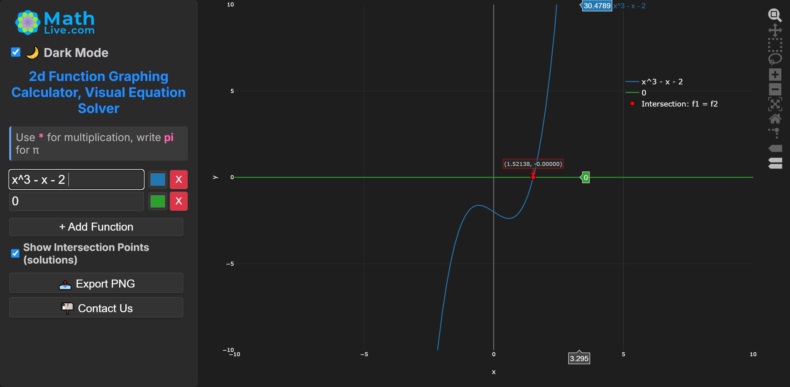
Worked Example: Solve \(x^3 - x - 2 = 0\)
1) Define: \( f(x) = x^3 - x - 2 \).
2) Choose an interval \([a,b]\) with opposite signs: \( a = 1,\; b = 2 \). Then \( f(1) = 1 - 1 - 2 = -2 \) (negative), \( f(2) = 8 - 2 - 2 = 4 \) (positive). Since the signs differ, a root lies in \([1,2]\).
3) Iterate (Bisection): at each step, take the midpoint \( m = \dfrac{a+b}{2} \) and keep the half-interval where the sign changes.
| Step | \(a\) | \(b\) | \(m=\frac{a+b}{2}\) | \(f(m)\) | Keep |
|---|---|---|---|---|---|
| 1 | 1.0000 | 2.0000 | 1.5000 | \(f(1.5)=-0.125\) | [1.5, 2] |
| 2 | 1.5000 | 2.0000 | 1.7500 | \(f(1.75)\approx 1.609\) | [1.5, 1.75] |
| 3 | 1.5000 | 1.7500 | 1.6250 | \(f(1.625)\approx 0.666\) | [1.5, 1.625] |
| 4 | 1.5000 | 1.6250 | 1.5625 | \(f(1.5625)\approx 0.249\) | [1.5, 1.5625] |
Continuing in this way shrinks the interval around the root. After several iterations, $$x \approx 1.52138 \quad \text{(to five decimal places).}$$
Stopping criterion: stop when \(b-a\) is below a chosen tolerance when \(|f(m)|\) is sufficiently small. MathLive uses tolerance = \(10^{-12}\).
Links: MathLive.com